Cartpole Problem

Competative Performance with Particle Swarm Optimisation

Adam Price

June 23rd 2020

OpenAI’s CartPole problem is a staple in reinforcement learning, it serves as a benchmark that many of RL’s most advanced algorithms have been applied to. However, it isn’t only RL algorithms that can solve control problems. In this article, I will give an overview of particle swarm optimisation (PSO); how it can be applied to control problems and how it compares to deep Q-learning.

If you want to follow along with all of the code I produced for this post, it can be seen in this Jupyter notebook.

What is Particle Swarm Optimisation?

Particle swarm optimisation is a metaheuristic optimisation algorithm. Metaheuristic algorithms search for a maximum (or minimum) value of a given function, without the need of much prior knowledge of the function.

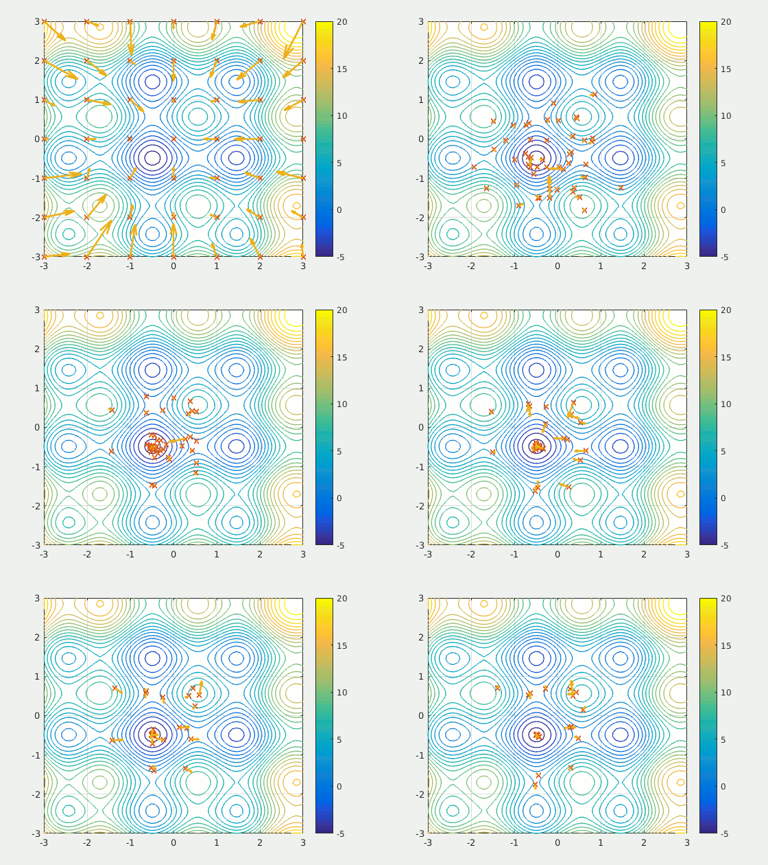
Particle swarm optimises by moving particles through the search space. At discrete time steps, the particles are evaluated by using their location as a parameter of a fitness function (the function being optimised). The particles are then drawn towards both the global best solution (found by another particle in the swarm) and the best solution that they found.

PSO is gradient-free, which makes it quick to perform updates (useful when using a large population), however, it cant guarantee convergences to a local minimum (or maximum).

The individual particle’s velocity is controlled by 3 parameters:

• Global Weight (φᵍ) — attraction to the location of the global best solution.
• Local Weight (φˡ) — attraction to the location of the particles best solution.
• Local Weight (φˡ) — attraction to the location of the particles best solution.

We also need to provide the algorithm with; search space bounds (to stop the particles leaving the search space); a fitness function to optimise; and the number of particles to use.

Applying PSO to the CartPole Problem

The PSO framework we have created is very flexible. We only need to pass it a function f(θ), where θ is a parameter vector, and it will attempt to find θ that maximises the function.

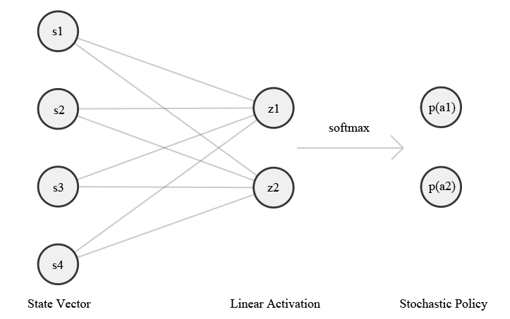
To apply PSO to the CartPole problem, we need to use the particle’s location, in the search space, to generate a policy for the CartPole problem to follow. To do this, we use a linear network with two outputs that are past through the softmax function to create a stochastic policy.

Using the current state of the CartPole as the input layer and the location of a particle as weights, we produce a probability of selecting two actions (moving the cart left or right).

The fitness of the particle’s position is given by the performance (reward accumulation) of the policy. The initial state of the environment is random, so we have to evaluate the policy for multiple episodes to get an estimate of the policies quality. This could prove inefficient in some environment, but running CartPole to termination is very computationally cheap.

With all this set up we can begin an experiment!

Performance

When we ran the script above, we found that the CartPole problem was solved in an average of 2.4 iterations. Compared to other learning methods, this is exceptionally few iterations. Well optimised deep Q-learning methods tend to require around 30 iterations to solve CartPole.

So has PSO outperformed deep learning methods?

We need to keep in mind the swarm used. In a standard RL implementation, a single agent is used, it can only run a single episode each iteration. Our swarm effectively runs 15 episodes each iteration so it could be argued that PSO actually took 36 (2.4*15) episodes to solve the problem. Which is about on par with deep Q.

On the other hand, the single RL agent requires far more computation than a single swarm agent. In the case of a deep learning implementation, there could be 1000s of weights being updated each time step. In contrast, our entire swarm is optimising 120 (8*15) weights between episodes.

Perhaps we could compare methods by the time it takes them to find solutions? But then we would need to consider computer architecture. Deep methods benefit from GPU’s whereas, PSO would benefit from parallel computing.

Ultimately, it very difficult to accurately compare such different methods. But, I do think that we have managed to present a good case for further investigation of metaheuristics in control.